44 excel data labels every other point
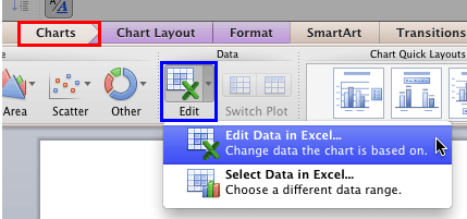
How to create Custom Data Labels in Excel Charts - Efficiency 365 Create the chart as usual. Add default data labels. Click on each unwanted label (using slow double click) and delete it. Select each item where you want the custom label one at a time. Press F2 to move focus to the Formula editing box. Type the equal to sign. Now click on the cell which contains the appropriate label. Add or remove data labels in a chart - support.microsoft.com To label one data point, after clicking the series, click that data point. In the upper right corner, next to the chart, click Add Chart Element > Data Labels. To change the location, click the arrow, and choose an option. If you want to show your data label inside a text bubble shape, click Data Callout.
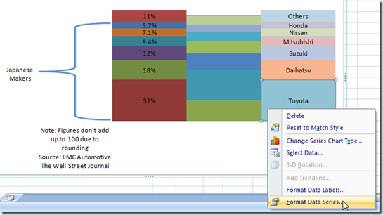
Apply Custom Data Labels to Charted Points - Peltier Tech Double click on the label to highlight the text of the label, or just click once to insert the cursor into the existing text. Type the text you want to display in the label, and press the Enter key. Repeat for all of your custom data labels. This could get tedious, and you run the risk of typing the wrong text for the wrong label (I initially ...
Excel data labels every other point
Show Data Label in Excel Chart Only When Data Point is selected/hovered ... Hi there, Does anyone know if it is possible to set Data Labels that are pointing to a range of selected cells and not just coming natively from the data. ... Show Data Label in Excel Chart Only When Data Point is selected/hovered over; Show Data Label in Excel Chart Only When Data Point is selected/hovered over. Discussion Options. Add a DATA LABEL to ONE POINT on a chart in Excel Steps shown in the video above: Click on the chart line to add the data point to. All the data points will be highlighted. Click again on the single point that you want to add a data label to. Right-click and select ' Add data label ' This is the key step! Right-click again on the data point itself (not the label) and select ' Format data label '. In Excel graphs, is it possible to have fewer markers, like one ... - Quora The most straightforward (and manual) approach is to create your graph and selectively right-click on each data point you want to erase and set the 'marker' option to 'none' one data point at a time. This is pretty inelegant and not so useful for a chart that has many data points, or is frequently updated.
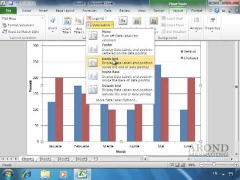
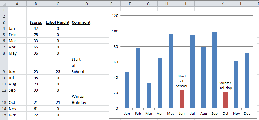
Excel data labels every other point. Solved: why are some data labels not showing? - Power BI Please use other data to create the same visualization, turn on the data labels as the link given by @Sean. After that, please check if all data labels show. If it is, your visualization will work fine. If you have other problem, please let me know. Best Regards, Angelia Message 3 of 4 95,242 Views 0 Reply fiveone Helper II Adding rich data labels to charts in Excel 2013 | Microsoft 365 Blog Putting a data label into a shape can add another type of visual emphasis. To add a data label in a shape, select the data point of interest, then right-click it to pull up the context menu. Click Add Data Label, then click Add Data Callout . The result is that your data label will appear in a graphical callout. Chart shows too many data labels | MrExcel Message Board So went to Chart - Chart Options - Data Labels and clicked box to show labels What happens is that the label "apples" is applied to each data point in the line of apples , and the same for every other "fruit". So I get a 60 labels in the chart. I would like to indicate this line is apples, this one is oranges... 1 label / line Quick Tip: Excel 2013 offers flexible data labels | TechRepublic right-click and choose Insert Data Label Field. In the next dialog, select [Cell] Choose Cell. When Excel displays the source dialog, click the cell that contains the MIN () function, and click OK....
Display every "n" th data label in graphs - Microsoft Community If the full chart labels are in column A, starting in cell A1, then you can use this formula to create a range with only every fifth label in another column: =IF (MOD (ROW (),5)=0,A1,"") cheers, teylyn ___________________ cheers, teylyn Community Moderator Report abuse 1 person found this reply helpful · Was this reply helpful? Yes Excel charts: add title, customize chart axis, legend and data labels Depending on where you want to focus your users' attention, you can add labels to one data series, all the series, or individual data points. Click the data series you want to label. To add a label to one data point, click that data point after selecting the series. Click the Chart Elements button, and select the Data Labels option. How to add data labels from different column in an Excel chart? Right click the data series in the chart, and select Add Data Labels > Add Data Labels from the context menu to add data labels. 2. Click any data label to select all data labels, and then click the specified data label to select it only in the chart. 3. How to Add Labels to Scatterplot Points in Excel - Statology Step 3: Add Labels to Points Next, click anywhere on the chart until a green plus (+) sign appears in the top right corner. Then click Data Labels, then click More Options… In the Format Data Labels window that appears on the right of the screen, uncheck the box next to Y Value and check the box next to Value From Cells.
Add Custom Labels to x-y Scatter plot in Excel Step 1: Select the Data, INSERT -> Recommended Charts -> Scatter chart (3 rd chart will be scatter chart) Let the plotted scatter chart be. Step 2: Click the + symbol and add data labels by clicking it as shown below. Step 3: Now we need to add the flavor names to the label. Now right click on the label and click format data labels. Prevent Overlapping Data Labels in Excel Charts - Peltier Tech Overlapping Data Labels Data labels are terribly tedious to apply to slope charts, since these labels have to be positioned to the left of the first point and to the right of the last point of each series. This means the labels have to be tediously selected one by one, even to apply "standard" alignments. How to Label Only Every Nth Data Point in #Tableau Here are the four simple steps needed to do this: Create an integer parameter called [Nth label] Crete a calculated field called [Index] = index () Create a calculated field called [Keeper] = ( [Index]+ ( [Nth label]-1))% [Nth label] As shown in Figure 4, create a calculated field that holds the values you want to display. How to Change Excel Chart Data Labels to Custom Values? - Chandoo.org Go to Formula bar, press = and point to the cell where the data label for that chart data point is defined. Repeat the process for all other data labels, one after another. See the screencast. Points to note: This approach works for one data label at a time. So if you have a large chart, you are in for a lot of clicks and manic mouse maneuvering.
MS Excel 2010 / How to remove data labels from the chart - YouTube
Dynamically Label Excel Chart Series Lines - My Online Training Hub Step 1: Duplicate the Series. The first trick here is that we have 2 series for each region; one for the line and one for the label, as you can see in the table below: Select columns B:J and insert a line chart (do not include column A). To modify the axis so the Year and Month labels are nested; right-click the chart > Select Data > Edit the ...

Business Diary: October 2011
show every other data label | MrExcel Message Board I have a chart with a number of data points and when I show all of the data labels, they overwrite each other. It's not necessary to see every one, but I need some data labels at regular intervals and I need the final data label. The chart updates frequently, so I don't want to be adding and removing data labels manually.
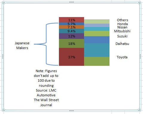
Creating Excel Stacked Column Chart Label Leader Lines/Spines - Excel Dashboard Templates
Excel 2016 VBA Display every nth Data Label on Chart Click on the bar you want to labeled twice before Add Data Labels. Click on the label, then right click and select Format Data Labels. Check the Category Name and uncheck Value. A little research before asking can save you a lot of time. Share answered Nov 7, 2017 at 13:15 user8753746 Add a comment

Excel Chart - Do not Hide Horizontal Data Label - Stack Overflow
Charting every second data point - Excel Help Forum If you want to chart only every other data point, then build a helper table that has only every other data value, then build the chart off that table. See attached on how to build the helper table. Use =INDEX (A:A,ROW ()*2-2) copy right and down. cheers Attached Files Copy of Chart.xls (27.5 KB, 18 views) Download Register To Reply
:max_bytes(150000):strip_icc()/015_5-how-to-create-a-scatter-plot-in-excel-hl-c260b9d91cd94c20ac15801ac139e0f8.jpg)
How to Create a Scatter Plot in Excel
Excel, giving data labels to only the top/bottom X% values 1) Create a data set next to your original series column with only the values you want labels for (again, this can be formula driven to only select the top / bottom n values). See column D below. 2) Add this data series to the chart and show the data labels. 3) Set the line color to No Line, so that it does not appear! 4) Volia! See Below! Share
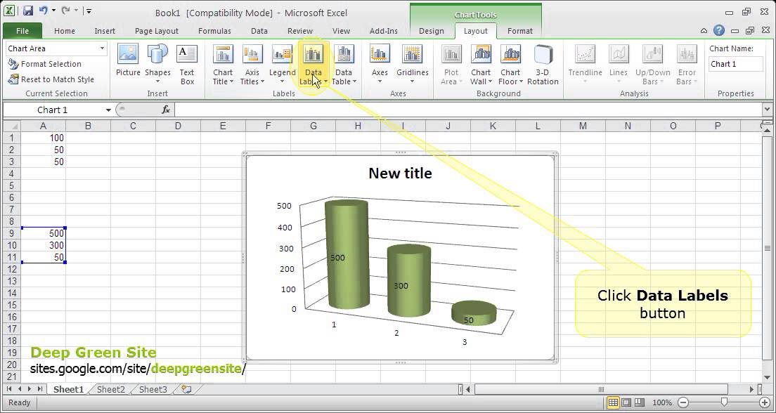
Using Excel 2010 - Add Data Labels - YouTube
Change the display of chart axes - support.microsoft.com On the Format tab, in the Current Selection group, click the arrow in the Chart Elements box, and then click the horizontal (category) axis. On the Design tab, in the Data group, click Select Data. In the Select Data Source dialog box, under Horizontal (Categories) Axis Labels, click Edit.

How to Create Progress Charts (Bar and Circle) in Excel - Automate Excel
Excel Charts: Dynamic Label positioning of line series - Xelplus Select your chart and go to the Format tab, click on the drop-down menu at the upper left-hand portion and select Series "Actual". Go to Layout tab, select Data Labels > Right. Right mouse click on the data label displayed on the chart. Select Format Data Labels. Under the Label Options, show the Series Name and untick the Value.

Format Number Options for Chart Data Labels in Excel 2011 for Mac
Find, label and highlight a certain data point in Excel ... - Ablebits To display both x and y values, right-click the label, click Format Data Labels…, select the X Value and Y value boxes, and set the Separator of your choosing: Label the data point by name In addition to or instead of the x and y values, you can show the month name on the label.
:max_bytes(150000):strip_icc()/PreparetheWorksheet2-5a5a9b290c1a82003713146b.jpg)
How to Make Labels from Excel
How to Use Cell Values for Excel Chart Labels - How-To Geek Select the chart, choose the "Chart Elements" option, click the "Data Labels" arrow, and then "More Options.". Uncheck the "Value" box and check the "Value From Cells" box. Select cells C2:C6 to use for the data label range and then click the "OK" button. The values from these cells are now used for the chart data labels.
Excel Bar Charts - Clustered, Stacked - Template - Automate Excel
In Excel graphs, is it possible to have fewer markers, like one ... - Quora The most straightforward (and manual) approach is to create your graph and selectively right-click on each data point you want to erase and set the 'marker' option to 'none' one data point at a time. This is pretty inelegant and not so useful for a chart that has many data points, or is frequently updated.

Import Web Data to Excel - Excel, the wise way
Add a DATA LABEL to ONE POINT on a chart in Excel Steps shown in the video above: Click on the chart line to add the data point to. All the data points will be highlighted. Click again on the single point that you want to add a data label to. Right-click and select ' Add data label ' This is the key step! Right-click again on the data point itself (not the label) and select ' Format data label '.
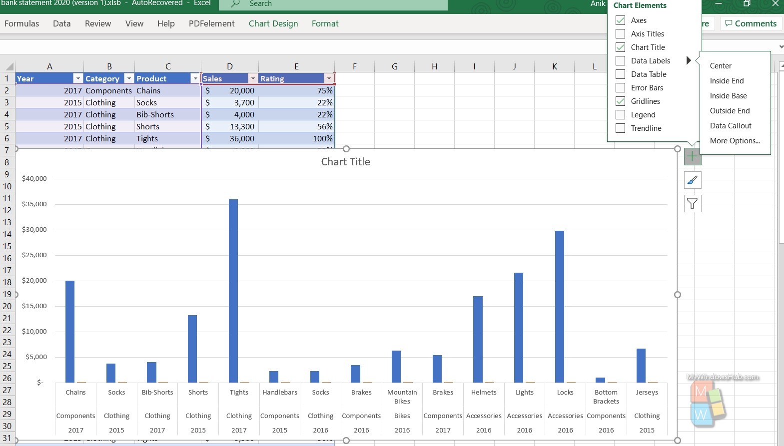
How To Show Or Hide Data Labels On MS Excel? | My Windows Hub
Show Data Label in Excel Chart Only When Data Point is selected/hovered ... Hi there, Does anyone know if it is possible to set Data Labels that are pointing to a range of selected cells and not just coming natively from the data. ... Show Data Label in Excel Chart Only When Data Point is selected/hovered over; Show Data Label in Excel Chart Only When Data Point is selected/hovered over. Discussion Options.
Format Number Options for Chart Data Labels in Excel 2011 for Mac

Adding Colored Regions to Excel Charts - Duke Libraries Center for Data and Visualization Sciences
Creating Excel Stacked Column Chart Label Leader Lines/Spines - Excel Dashboard Templates

33 How To Label Points In Excel - Label Design Ideas 2020

8 Labels Per Sheet Template Word - Sample Professional Template
Post a Comment for "44 excel data labels every other point"