40 pivot table multiple row labels

How to make row labels on same line in pivot table? - ExtendOffice Make row labels on same line with PivotTable Options You can also go to the PivotTable Options dialog box to set an option to finish this operation. 1. Click any one cell in the pivot table, and right click to choose PivotTable Options, see screenshot: 2. Repeat item labels in a PivotTable - support.microsoft.com Right-click the row or column label you want to repeat, and click Field Settings. Click the Layout & Print tab, and check the Repeat item labels box. Make sure Show item labels in tabular form is selected. When you edit any of the repeated labels, the changes you make are applied to all other cells with the same label.

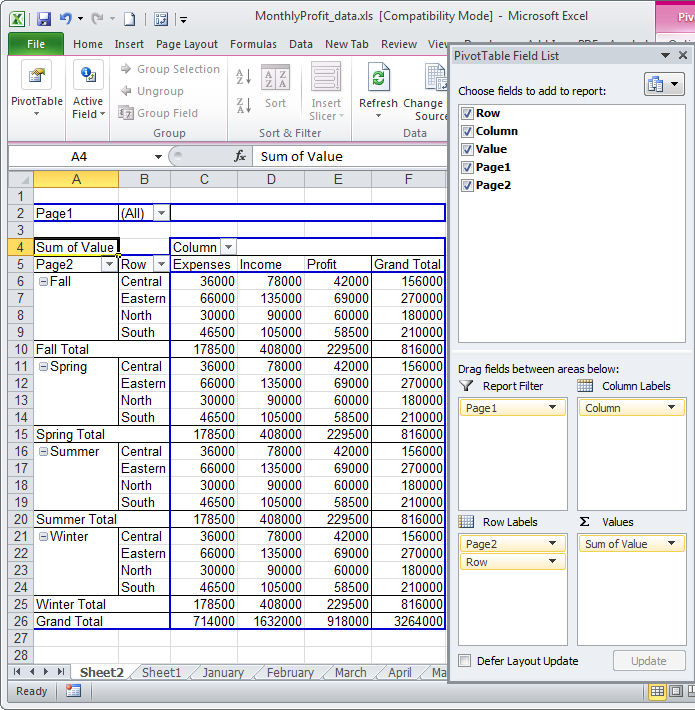
Pivot table row labels in separate columns - AuditExcel.co.za Our preference is rather that the pivot tables are shown in tabular form (all columns separated and next to each other). You can do this by changing the report format. So when you click in the Pivot Table and click on the DESIGN tab one of the options is the Report Layout. Click on this and change it to Tabular form.

Pivot table multiple row labels

Multiple row labels on one row in Pivot table | MrExcel ... Nov 14, 2002 · I figured it out - Right click on your pivot table and choose pivot table options/display. Click on “Classic PivotTable layout” Then click on where it is subtotaling your row label and uncheck the subtotal option. D dudeshane0 New Member Joined Oct 23, 2014 Messages 1 Jan 19, 2015 #6 Gerald Higgins said: How to rename group or row labels in Excel PivotTable? - ExtendOffice 1. Click at the PivotTable, then click Analyze tab and go to the Active Field textbox. 2. Now in the Active Field textbox, the active field name is displayed, you can change it in the textbox. You can change other Row Labels name by clicking the relative fields in the PivotTable, then rename it in the Active Field textbox. Excel: How to Apply Multiple Filters to Pivot Table at Once Example: Apply Multiple Filters to Excel Pivot Table. Suppose we have the following pivot table in Excel that shows the total sales of various products: Now suppose we click the dropdown arrow next to Row Labels, then click Label Filters, then click Contains: And suppose we choose to filter for rows that contain "shirt" in the row label:

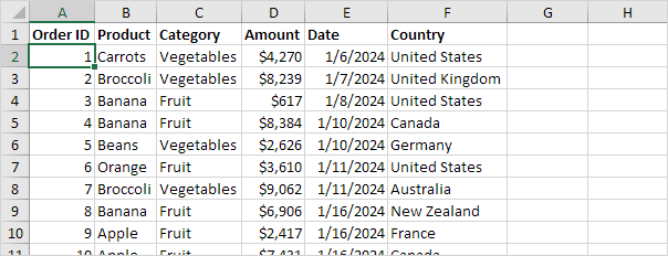
Pivot table multiple row labels. Duplicate Items Appear in Pivot Table - Excel Pivot Tables In Row 2 of the new column, enter the formula =TRIM(C2). Copy the formula down to the last row of data in the source table. If the source data is stored in an Excel Table, the formula should copy down automatically. Refresh the pivot table ; Remove the City field from the pivot table, and add the CityName field to replace it. _____ row - Excel pivot table: How to transpose multiple value in column to a ... Here's the pivot table I have in excel: I have a list of website with their emails address. Sometime you have one email per website, sometime you have 3 emails per website. I want to transpose the multiple emails I have for one website that are in column Email 1 into multiple field such as Email 1, Email 2, Email 3 for EACH corresponding websites. Pivot Table Multiple Row Labels? [SOLVED] - excelforum.com You can, of course, create a pivot table that sums the values just at the owner level. then, create a second pivot table that sums the values at the Engineer level. If you need to present this data in a contiguous table, you can create a new Excel table and reference to the pivot table values with formulas (=PivotTableSheet!A1) cheers Microsoft MVP Multi-level Pivot Table in Excel (In Easy Steps) - Excel Easy Multiple Row Fields First, insert a pivot table. Next, drag the following fields to the different areas. 1. Category field and Country field to the Rows area. 2. Amount field to the Values area. Below you can find the multi-level pivot table. Multiple Value Fields First, insert a pivot table. Next, drag the following fields to the different areas.

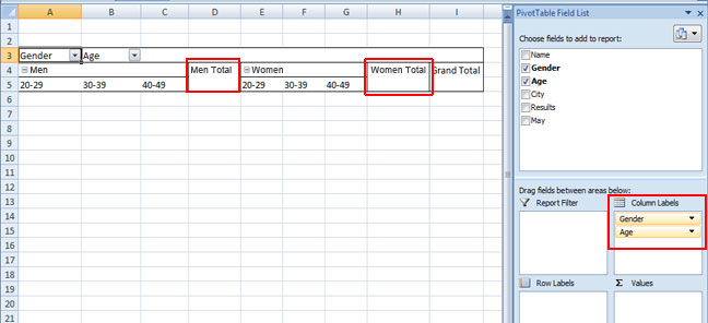
How to Filter Multiple Values in Pivot Table - OfficeTuts Excel When we click OK, we will have only LeBron James selected in our Pivot Table:. Filter with Slicers. Another way to filter multiple values in Pivot Table is to use Slicers.We will create another Pivot Table with the same data. Then we will place player, team, and conference in rows fields and the sum of points, rebounds, assists in the values field. Pivot table row labels side by side - Excel Tutorials - OfficeTuts Excel You can copy the following table and paste it into your worksheet as Match Destination Formatting. Now, let's create a pivot table ( Insert >> Tables >> Pivot Table) and check all the values in Pivot Table Fields. Fields should look like this. Right-click inside a pivot table and choose PivotTable Options…. Check data as shown on the image below. Apply Multiple Filters on a Pivot Field - Pivot Table Right-click any cell in the pivot table, and click PivotTable Options. Click the Totals & Filters tab. Under Filters, add a check mark to 'Allow multiple filters per field.'. Click OK. Now you can apply both a Label filter and a Value filter to the OrderMth field, and both will be retained. In the screen shot below, both the Label filter ... How to Use Excel Pivot Table Label Filters - Contextures Excel Tips Right-click a cell in the pivot table, and click PivotTable Options. In the PivotTable Options dialog box, click the Totals & Filters tab In the Filters section, add a check mark to 'Allow multiple filters per field.' Click the OK button, to apply the setting and close the dialog box. Quick Way to Hide or Show Pivot Items

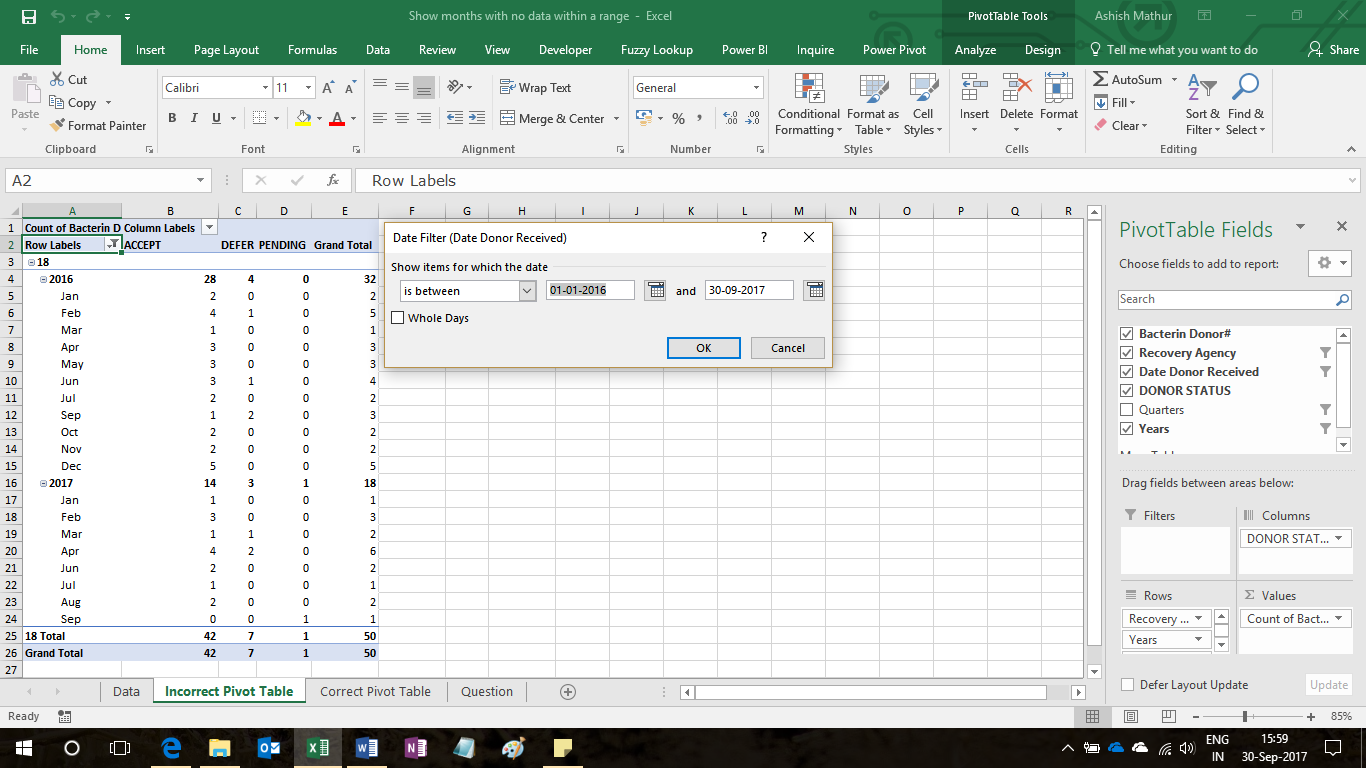
Combining two+ Columns to form one Row label column in Pivot Table Hello, I have multiple sets of data that occur in 2 column increments. The first column is a list of part numbers, the second is their value for that month. I want a pivot table that combines all of the first columns into one master row label of Part numbers and then the values will be listed out in each subsequent column. If a particular month doesn't have a part number in its data, then it ... How to filter date range in an Excel Pivot Table? - ExtendOffice Go to the pivot table, you will see the Date field is added as report filter above the pivot table. 3. Please click the arrow beside (All), check Select Multiple Items option in the drop-down list, next check dates you will filter out, and finally click the OK button. See screenshot: Now you have filtered date range in the pivot table. Automate Pivot Table with Python (Create, Filter and Extract) 22.05.2021 · Photo by Jasmine Huang on Unsplash. In Automate Excel with Python, the concepts of the Excel Object Model which contain Objects, Properties, Methods and Events are shared.The tricks to access the Objects, Properties, and Methods in Excel with Python pywin32 library are also explained with examples.. Now, let us leverage the automation of Excel report … How to make row labels on same line in pivot table? - ExtendOffice Make row labels on same line with PivotTable Options You can also go to the PivotTable Options dialog box to set an option to finish this operation. 1. Click any one cell in the pivot table, and right click to choose PivotTable Options, see screenshot: 2.

Group data in an Excel Pivot Table

Excel Pivot Table with multiple columns of data and each data … 17.04.2019 · Then I made multiple Pivot Tables, filling the Columns and Values Pivot Table Fields with one Category of each of your categories. This will produce a Pivot Table with 3 rows. The first row will read Column Labels with a filter dropdown. The second row will read all the possible values of the column. The third row will be the count of each ...

How to reset a custom pivot table row label

How to Move Excel Pivot Table Labels Quick Tricks 12.07.2021 · Change Order of Pivot Table Labels. When you add a field to the Row Label or Column Label area of the pivot table, its labels are usually sorted alphabetically. If you want the labels in a nonalphabetical order, you can manually move them, instead of using the Sort options. The following video shows 3 ways to manually move the labels, and the ...

Pivot Table Duplicate Row Labels

How to repeat row labels for group in pivot table? - ExtendOffice Except repeating the row labels for the entire pivot table, you can also apply the feature to a specific field in the pivot table only. 1. Firstly, you need to expand the row labels as outline form as above steps shows, and click one row label which you want to repeat in your pivot table. 2.

How to use Excel Pivot Tables | PowerPoint Presentation

How to Add a Field to a Pivot Table: 14 Steps (with Pictures) 28.03.2019 · Grouping your data into a pivot table allows you to arrange the information as you like and provides a way to illustrate the conclusions you can make from analyzing the data. Adding a field to a pivot table gives you another way to refine, sort and filter the data. The field you choose to add to your pivot table can be used as a row label, column label or even a …

Frequency Distribution in Excel - Easy Excel Tutorial

how can i use a pivot table with multiple row labels in formulas but if the case is multiple row labels pivot, i'am having problem since the first label values (and second, third, etc) repeats only once in the column and the cells below are blank. my solution is: copy-paste values of pivot data to another range and fill in the blanks in the columns with the values from above cells.

excel pivot table - multiple label filters - Stack Overflow

Can't Move Multiple Measures to Row Labels With your powerpivot table, open the Pivot Table Field List (the old kind)...add the two measure to the Values Area. They will show in columns but there will now be a Sigma Values in the Column Labels. Move the Sigma Values to Row Lables and you should be good. Close the Pivot Table Field list and continue using the powerpivot interface.

Pivot table row labels in separate columns • AuditExcel.co.za

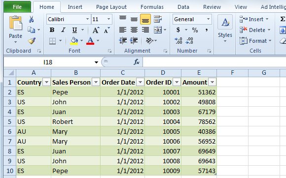
Automatic Row And Column Pivot Table Labels - How To Excel At Excel Select the data set you want to use for your table The first thing to do is put your cursor somewhere in your data list Select the Insert Tab Hit Pivot Table icon Next select Pivot Table option Select a table or range option Select to put your Table on a New Worksheet or on the current one, for this tutorial select the first option Click Ok

Advanced Excel - Pivot Table Recommendations - Tutorial Desk

Consolidate Multiple Worksheets into Excel Pivot Tables 20.06.2021 · In this tutorial we will show you how to consolidate multiple worksheets into a Pivot table using Excel.. If the data is arranged properly, then you can do that. Most of the time, when you create a Pivot table in Excel 2013 or Excel 2016, you’ll use a list or an Excel table.. There might be some different worksheets (or workbooks) that you have in your collection with …

Pivot table row labels side by side | Pivot table, Labels, Sides

Pivot Table Row Labels In the Same Line - Beat Excel! Then navigate to "Layout & Print" tab and click on "Show item in tabular form" option. Do this procedure also for "Dealer" field and your table will look like this: If you also want dealer names to repeat on each row, reopen "Dealer field settings and check "Repear item labels" option in "Layout & Print" tab.

Pivot Table Duplicate Row Labels

Pivot table when same record appears multiple times - Stack Overflow If I create a pivot table to count the number of restaurants by each dining style I'll get an accurate result since the Dining Style field is multi-select. Row Labels Count of Dining Style Dine-in 3 Take Out 2 However, if I create pivot table to summarize the count by restaurant type I'll get an inaccurate result.

Sorting to your Pivot table row labels in custom order [quick tip] » Chandoo.org - Learn Excel ...

Ranking to a Pivot Table with multiple Row Labels I have a pivot table with multiple Row Labels: Team and Player. I then have a bunch of stat categories under Values, one of which is 'Pts' I have the table sorted by Pts, but I need a 'Ranking' column I created a second Pts column and used 'Show Values As - Rank Largest to Smallest', but it's not working. It's showing up as '1' for all columns, regardless of whether or not I pick 'Team' or ...

[5 Steps] How To Make Ranking Charts With Excel Pivot Tables - Moz

How to make row labels on same line in pivot table? Make row labels on same line with PivotTable Options You can also go to the PivotTable Options dialog box to set an option to finish this operation. 1. Click any one cell in the pivot table, and right click to choose PivotTable Options, see screenshot: 2.

Lesson 55: Pivot Table Column Labels - Swotster

How to Add Rows to a Pivot Table: 9 Steps (with Pictures) 15.02.2022 · Click the tab that contains the data you're using in your pivot table, and make sure it contains the data you want to use to create your new row. For example, if you want to add a row for a specific purchase, make sure that purchase is …

Choosing PivotTable Layouts | Microsoft Excel - Pivot Tables

101 Advanced Pivot Table Tips And Tricks You Need To Know 25.04.2022 · With all options unchecked the pivot table is empty of row headers, banded rows, column headers and ... Tabular form will not be in a hierarchical structure and each Row field will be in a separate column in the pivot table. Repeat All Item Labels. You can repeat all your pivot tables item labels by going to the Design tab and selecting the Report Layout button under the …

Pivot Table Duplicate Row Labels

Pivot Table Error: Excel Field Names Not Valid 20.10.2009 · If there are any merged cells in the heading row, unmerge them, and add a heading in each separate cell. Select each heading cell and check its contents in the formula bar; text from one heading may overlap a blank cell beside it. In this example, the Product Name heading overlapped the empty heading cell beside it. If there are no blank heading cells, and you are …

How To Find And Remove Duplicates In A Pivot Table - MS Excel | Excel In Excel

Excel Pivot Table Multiple Consolidation Ranges 15.11.2021 · Pivot Table from Multiple Consolidation Ranges. To open the PivotTable and PivotChart Wizard, select any cell on a worksheet, then press Alt+D, then press P. That shortcut is used because in older versions of Excel, the wizard was listed on the Data menu, as the PivotTable and PivotChart Report command. Click Multiple consolidation ranges, then click …

33 Pivot Table Blank Row Label - Labels Database 2020

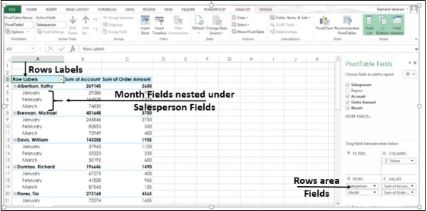
multiple fields as row labels on the same level in pivot ... Jan 12, 2018 · multiple fields as row labels on the same level in pivot table Excel 2016 I am using Excel 2016. I have data that lists product models along with relevant data and also production volumes by month. Part of the relevant data are about 5 common part columns with the part # that applies to each model under the appropriate column.

Excel pivot table categorical variables the same in multiple columns (histogram) - Super User

Excel: How to Apply Multiple Filters to Pivot Table at Once Example: Apply Multiple Filters to Excel Pivot Table. Suppose we have the following pivot table in Excel that shows the total sales of various products: Now suppose we click the dropdown arrow next to Row Labels, then click Label Filters, then click Contains: And suppose we choose to filter for rows that contain "shirt" in the row label:

Share :