43 how to display data labels above the columns in excel

Format Chart Axis in Excel - Axis Options Now we can insert a column chart from this data. This will be the inserted chart. You can check the blog on how to insert a chart in excel. Analyzing Format Axis Pane Right-click on the Vertical Axis of this chart and select the "Format Axis" option from the shortcut menu. This will open up the format axis pane at the right of your excel interface. Guide: How to Name Column in Excel | Indeed.com Choose the "Advanced" option in the left navigation pane to the Display options for this worksheet section. Uncheck the box for "Show row and column headers." When you return to the worksheet, the column title row is the only column header that would be visible. To make the default column header re-appear, you can re-check the box. 2.

Headings Missing in Excel: How to Show Row Numbers & Column Letters! Select all worksheets (hold down the Ctrl key and click on the tabs or alternatively press and hold the Shift key and click on the sheet tabs - that way you also select the sheets in-between). Now, do the steps as shown before: Go to the View ribbon and click on "Headings". Do you want to boost your productivity in Excel?

How to display data labels above the columns in excel

5 New Charts to Visually Display Data in Excel 2019 - dummies Place text labels describing the data sets above the data. Select the data sets and their column labels. Click Insert → Insert Statistic Chart → Box and Whisker. Format the chart as desired. Box and whisker charts are visually similar to stock price charts, which Excel can also create, but the meaning is very different. chandoo.org › wp › change-data-labels-in-chartsHow to Change Excel Chart Data Labels to Custom Values? May 05, 2010 · Now, click on any data label. This will select “all” data labels. Now click once again. At this point excel will select only one data label. Go to Formula bar, press = and point to the cell where the data label for that chart data point is defined. Repeat the process for all other data labels, one after another. See the screencast. How to Add a Header in Microsoft Excel - How-To Geek In Excel's ribbon at the top, click the "Insert" tab. In the "Insert" tab, click Text > Header & Footer. Your worksheet's view will immediately change, and you can now start adding your header. At the top of your worksheet, you have a left, middle, and right section to specify your header's content. Click each section and add your ...

How to display data labels above the columns in excel. How to Use Excel Pivot Table Label Filters Watch the steps in this short video, and the written instructions are below the video. Play. To change the Pivot Table option to allow multiple filters: Right-click a cell in the pivot table, and click PivotTable Options. Click the Totals & Filters tab Under Filters, add a check mark to 'Allow multiple filters per field.'. How to Add Labels to Scatterplot Points in Excel - Statology Step 3: Add Labels to Points. Next, click anywhere on the chart until a green plus (+) sign appears in the top right corner. Then click Data Labels, then click More Options…. In the Format Data Labels window that appears on the right of the screen, uncheck the box next to Y Value and check the box next to Value From Cells. Excel Conditional Formatting Data Bars Select the cells that contain the data bars. On the Ribbon, click the Home tab In the Styles group, click Conditional Formating, and then click Manage Rules. In the list of rules, click your Data Bar rule, then click the Edit Rule button In the "Edit the Rule Description" section, the default settings are shown for Minimum and Maximum Columns and rows are labeled numerically - Office | Microsoft Docs To change this behavior, follow these steps: Start Microsoft Excel. On the Tools menu, click Options. Click the Formulas tab. Under Working with formulas, click to clear the R1C1 reference style check box (upper-left corner), and then click OK.

How To Change Excel's Group Outline Direction Settings Here are the steps to change the vertical or horizontal direction of Excel's Outline Groups: Select the Data Tab. Within the Outline group, click the dialog launcher button. The two checkboxes within the Direction section of the Settings Dialog box will allow you to control which direction your outline groups expand/collapse. Click the OK button. Excel 365 multiple columns with data, but all mixed up. How to sort so ... So I have an excel document that contains information on various software names and types, having used Text to Columns I have unsorted data running left to right that is not alphabetical. the row above and below will hold different data in the same cell. How can I sort several columns - up to 15 to display each title in the same column? Including Design Data in an Excel-format Bill of Materials (BOM) This feature has been used in certain versions of the example templates included in the software, to hide the Column = declarations. To display hidden rows or columns in Excel, select all cells in the template, then right-click anywhere on the sheet and choose the Unhidecommand. Mapping Project-Level, BOM Header Information linkedin-skill-assessments-quizzes/microsoft-excel-quiz.md at ... - GitHub Microsoft Excel Q1. Some of your data in Column C is displaying as hashtags (#) because the column is too narrow. How can you widen Column C just enough to show all the data? Right-click column C, select Format Cells, and then select Best-Fit. Right-click column C and select Best-Fit. Double-click column C.

How to Display Percentage in an Excel Graph (3 Methods) Select the Helper columns and click on the plus icon. Then go to the More Options via the right arrow beside the Data Labels. Select Chart on the Format Data Labels dialog box. Uncheck the Value option. Check the Value From Cells option. Then you have to select cell ranges to extract percentage values. How to Highlight Duplicates in Excel (6 Easy Ways) Every step will be similar to the above ones except for one thing. Here you have to select the whole single column. To do this simply click on the column header. We have clicked on column B. Follow the rest of the steps given above and the result for this is shown below. You can see that all the duplicates are highlighted. How to Show Percentages in Stacked Column Chart in Excel? Follow the below steps to show percentages in stacked column chart In Excel: Step 2: Select the entire data table. Step 3: To create a column chart in excel for your data table. Go to "Insert" >> "Column or Bar Chart" >> Select Stacked Column Chart. Step 4: Add Data labels to the chart. Goto "Chart Design" >> "Add Chart Element ... Solved: How to print excel datatable value from a column w... - Power ... Read the Column Heading in a variable In this case the variable is MyColumnHeading. You can give a name similar to your Excel column headings. Also you can use a loop if you want to read all headings. Then use that column heading variable to get its value. Below is an example to display the 1st item (actually 2nd) from the data table.

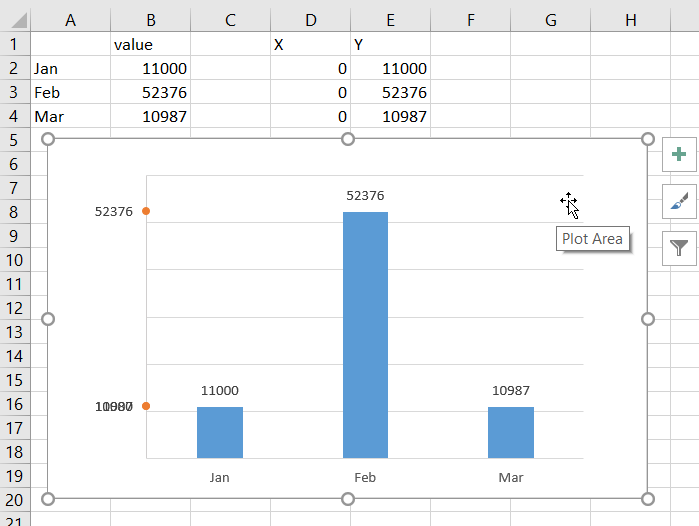
Is it possible to display the exact value on the y-axis on a - Microsoft Community

peltiertech.com › text-labels-on-horizontal-axis-in-eText Labels on a Horizontal Bar Chart in Excel - Peltier Tech Dec 21, 2010 · In this tutorial I’ll show how to use a combination bar-column chart, in which the bars show the survey results and the columns provide the text labels for the horizontal axis. The steps are essentially the same in Excel 2007 and in Excel 2003. I’ll show the charts from Excel 2007, and the different dialogs for both where applicable.

Quick Tip: Excel 2013 offers flexible data labels - TechRepublic

› analyze-large-data-setsExcel for Commerce | Analyze large data sets in Excel May 07, 2015 · Now that you have these calculated columns, you can use filters as you did above to find the top names in each year. Select Columns A:F, and in the HOME tab, under Sort & Filter, choose Filter. Now click the filter icon in cell F1 and select only the names of rank one (i.e. the #1 names of each sex of each year).

Which Excel chart should I use to display this complex data? - Quora

techcommunity.microsoft.com › t5 › excelCopy Data to Other Sheets' Columns Based on Criteria Sep 22, 2017 · The Orders sheet will have all the order data for an entire year. The Month sheets have the same columns as the Orders sheet excluding the Dept and Cost columns. Instead of one column for Dept there are 10 columns, one for each of the options. These columns will be populated with the cost of each option.

How-to Use Data Labels from a Range in an Excel Chart - Excel Dashboard Templates

› charts › dynamic-chart-dataCreate Dynamic Chart Data Labels with Slicers - Excel Campus Feb 10, 2016 · Step 3: Use the TEXT Function to Format the Labels. Typically a chart will display data labels based on the underlying source data for the chart. In Excel 2013 a new feature called “Value from Cells” was introduced. This feature allows us to specify the a range that we want to use for the labels.

Stop Excel Overlapping Columns on Second Axis for 3 Series

COLUMN Function - Formula, Uses, How to Use COLUMN in Excel The COLUMN function in Excel is a Lookup/Reference function. This function is useful for looking up and providing the column number of a given cell reference. For example, the formula =COLUMN (A10) returns 1, because column A is the first column. Formula =COLUMN ( [reference])

PPC Storytelling: How to Make an Excel Bubble Chart for PPC

How to Create Labels in Word from an Excel Spreadsheet In the File Explorer window that opens, navigate to the folder containing the Excel spreadsheet you created above. Double-click the spreadsheet to import it into your Word document. Word will open a Select Table window. Here, select the sheet that contains the label data. Tick mark the First row of data contains column headers option and select OK.

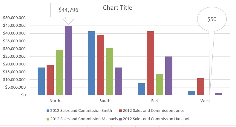
Display the data labels on this chart above the data markers

Excel Waterfall Chart: How to Create One That Doesn't Suck The first and last columns should be Total (start on the horizontal axis) and to set them as such, we have to double-click on each of them to open the Format Data Point task pane, and check the Set as total box. You can also right click the data point and select Set as Total from the list of menu options. Finally, we have our waterfall chart: 2.

Share :